Connected Components Algorithm

In this tutorial we are going to learn how to segment small objects in the image using the kornia implementation of the classic Computer Vision technique called Connected-component labelling (CCL).

%%capture
!pip install kornia
!pip install kornia-rs

import io

import requests


def download_image(url: str, filename: str = "") -> str:
    filename = url.split("/")[-1] if len(filename) == 0 else filename
    # Download
    bytesio = io.BytesIO(requests.get(url).content)
    # Save file
    with open(filename, "wb") as outfile:
        outfile.write(bytesio.getbuffer())

    return filename


url = "https://github.com/kornia/data/raw/main/cells_binary.png"
download_image(url)

'cells_binary.png'

from __future__ import annotations

import kornia as K
import matplotlib.pyplot as plt
import torch

We define utility functions to visualize the segmentation properly

def create_random_labels_map(classes: int) -> dict[int, tuple[int, int, int]]:
    labels_map: Dict[int, Tuple[int, int, int]] = {}
    for i in classes:
        labels_map[i] = torch.randint(0, 255, (3,))
    labels_map[0] = torch.zeros(3)
    return labels_map


def labels_to_image(img_labels: torch.Tensor, labels_map: Dict[int, Tuple[int, int, int]]) -> torch.Tensor:
    """Function that given an image with labels ids and their pixels intrensity mapping, creates a RGB
    representation for visualisation purposes."""
    assert len(img_labels.shape) == 2, img_labels.shape
    H, W = img_labels.shape
    out = torch.empty(3, H, W, dtype=torch.uint8)
    for label_id, label_val in labels_map.items():
        mask = img_labels == label_id
        for i in range(3):
            out[i].masked_fill_(mask, label_val[i])
    return out


def show_components(img, labels):
    color_ids = torch.unique(labels)
    labels_map = create_random_labels_map(color_ids)
    labels_img = labels_to_image(labels, labels_map)

    fig, (ax1, ax2) = plt.subplots(1, 2, figsize=(12, 12))

    # Showing Original Image
    ax1.imshow(img)
    ax1.axis("off")
    ax1.set_title("Orginal Image")

    # Showing Image after Component Labeling
    ax2.imshow(labels_img.permute(1, 2, 0).squeeze().numpy())
    ax2.axis("off")
    ax2.set_title("Component Labeling")

    plt.show()

We load the image using Kornia

img_t = K.io.load_image("cells_binary.png", K.io.ImageLoadType.GRAY32)[None, ...]

print(img_t.shape)

torch.Size([1, 1, 602, 602])

Apply the Connected-component labelling algorithm using the kornia.contrib.connected_components functionality. The num_iterations parameter will control the total number of iterations of the algorithm to finish until it converges to a solution.

labels_out = K.contrib.connected_components(img_t, num_iterations=150)
print(labels_out.shape)

torch.Size([1, 1, 602, 602])

show_components(img_t.numpy().squeeze(), labels_out.squeeze())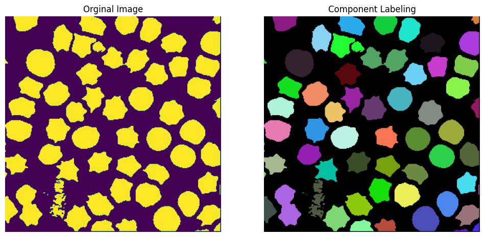

We can also explore the labels

print(torch.unique(labels_out))

tensor([     0.,  13235.,  24739.,  31039.,  32177.,  44349.,  59745.,  61289.,
         66209.,  69449.,  78869.,  94867., 101849., 102217., 102319., 115227.,
        115407., 137951., 138405., 150047., 158715., 162179., 170433., 170965.,
        174279., 177785., 182867., 210145., 212647., 215451., 216119., 221291.,
        222367., 226183., 226955., 248757., 252823., 255153., 263337., 265505.,
        270299., 270649., 277725., 282775., 296897., 298545., 299793., 300517.,
        313961., 316217., 321259., 322235., 335599., 337037., 340289., 347363.,
        352235., 352721., 360801., 360903., 360965., 361073., 361165., 361197.])